Neural Operators for PDEs

Mathematically, a neural operator $\mathcal{N}^\theta$ is defined as a mapping from an input domain function space $\mathcal{A}(\Omega_{\alpha};\mathbb{R}^{d_a})$ to an output target function space $\mathcal{U}(\Omega_{\alpha};\mathbb{R}^{d_u})$, represented as:

$$\mathcal{N}^{\theta}: \mathcal{A}(\Omega_{\alpha};\mathbb{R}^{d_a}) \rightarrow \mathcal{U}(\Omega_{\alpha};\mathbb{R}^{d_u})$$

where $\theta \in \Theta$ denotes the neural operator’s parameters, $\Omega_{\alpha} \subset \mathbb{R}^d$ (or a $d$-dimensional manifold $\mathcal{M}^d$) represents the spatial domain on which the functions are defined and $\alpha \in \mathscr{A}$ denotes the shape of the domain. The dimensions $d_a$ and $d_u$ denote the respective sizes of the input and output function spaces, often subspaces of Sobolev or Banach spaces.

Neural operators can be applied to various problems such as those described by continuous functions $C(\Omega;\mathbb{R}^{d_a})$ or Sobolev spaces $H^s(\Omega;\mathbb{R}^{d_a})$ for some $s \ge 0$. The neural operator $\mathcal{N}^{\theta}$ is an approximation of a true target operator $\mathcal{N}$, e.g., the solution operator of a partial differential equation (PDE) obtained by training on input-output function pairs $(a_i, u_i)_{i=1}^{m}$, where $a_i \in \mathcal{A}$ and $u_i = \mathcal{N}(a_i) \in \mathcal{U}$. These pairs could be simulation data representing a known, high-fidelity numerical approximation of the PDE.

My research on this topic aims at developing robust computational and mathematical frameworks for operator/PDE learning on arbitrary domains and enforcing known symmetries of the problem to enhance the data efficiency of these ideas.

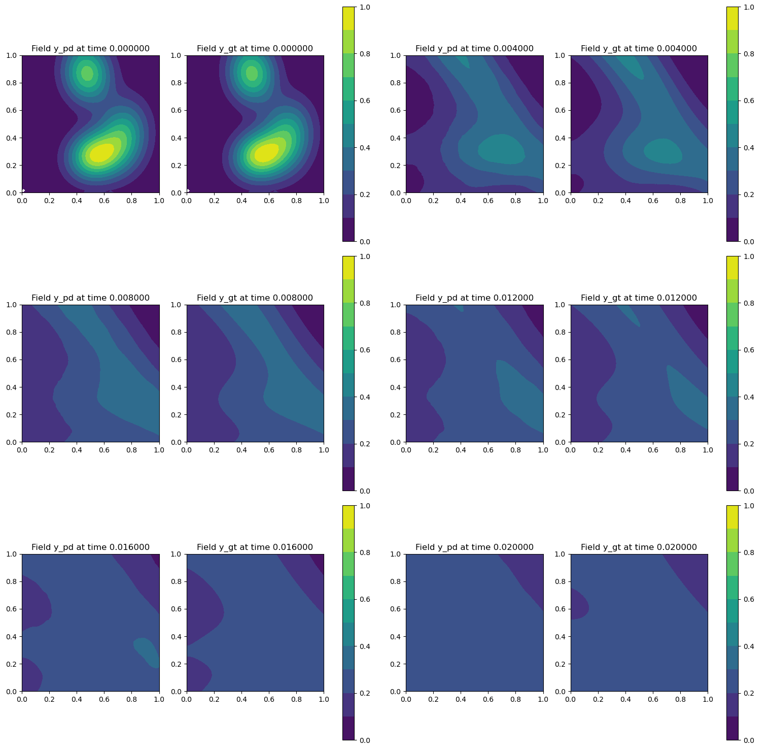
Figure 1: Neural operator prediction of solution to the anisotropic 2D heat equation compared with numerical solution.

These data-driven methods in scientific machine learning aim to avoid the computationally expensive numerical integration methods needed for large-scale simulations of PDE systems. This is especially beneficial for applications like domain optimization and precision medicine, where multiple PDEs need to be solved for varying parameters or domains, requiring significant computational resources. Neural operators learn mappings between high-dimensional (infinite-dimensional) function spaces, allowing them to generalize across a family of PDEs without retraining for varying parameters or conditions.

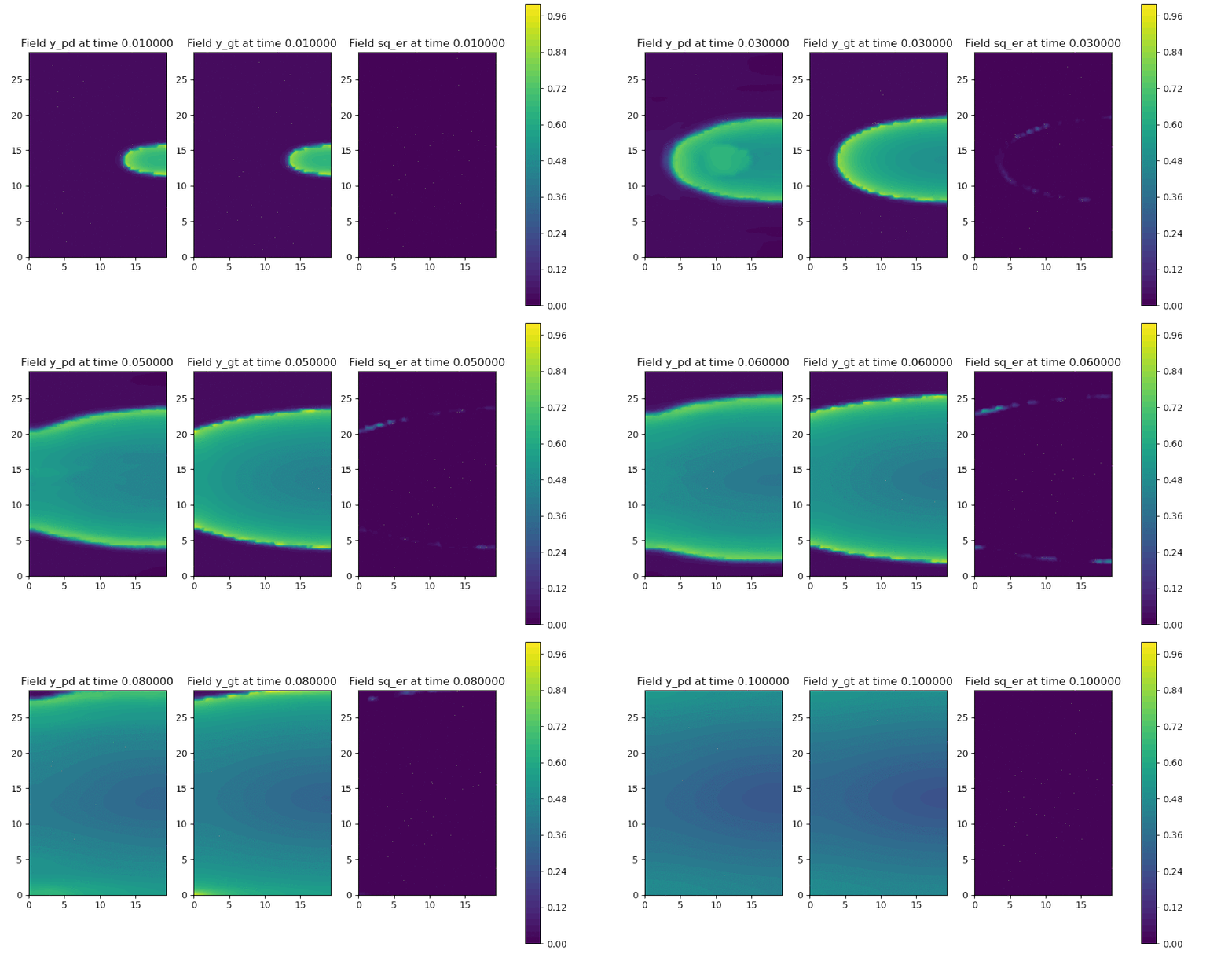
Figure 2: Neural operator vs. numerical solver for reaction-diffusion on anisotropic 2D rectangle.

In cardiac electrophysiology, for example, $\mathcal{A}$ might represent the space of initial electrical activation patterns across varying cardiac tissue geometries, whereas $\mathcal{U}$ could correspond to the resultant electrical potential fields over time. Below is an example of a prediction of cardiac electrophysiology dynamics on an unseen left atrial geometry and anisotropic fiber field:

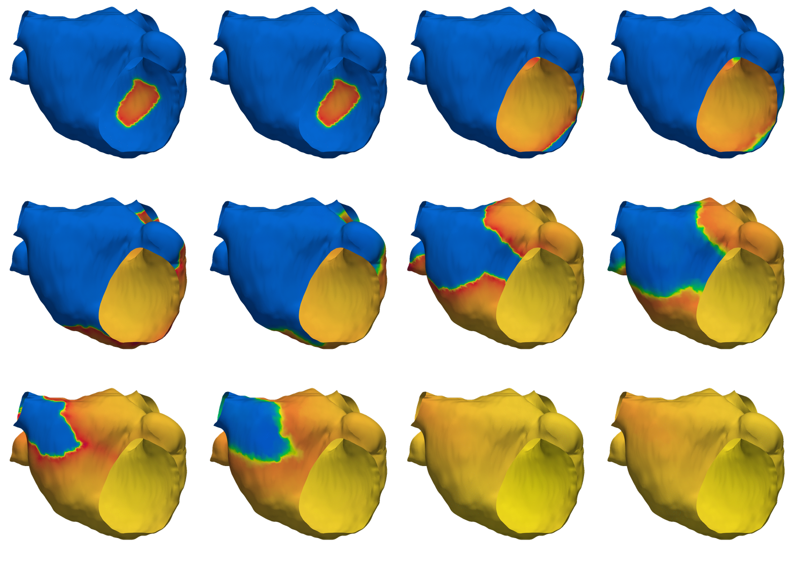
Figure 3: Cardiac Electrophysiology Simulation using Neural Operators (left: ground truth, right: prediction).

← Back