Chapter 7: Confidence Intervals
The current lecture deck has 83 PDF pages. The existing 18-page notes cover the chapter with explanations and additional practice. Sections below follow the slide order; finite-population sampling appears later in the notes. Questions and previously released solutions remain in their existing locations.
Practice and worked solutions
Page numbers refer to the PDF viewer, including repeated slide reveals. Use the links below or the navigation strip in either PDF to switch between notes and slides. Some mobile or embedded viewers open at page 1; if so, enter the page number shown here. Navigation sits above the original page; content, page order and existing page references are unchanged.
November 5 revision: notation follows the course slides; figures connect the equations to their meaning. Notes retain their existing page numbers. On a small screen, swipe a wide figure or open its full-size view.
Parameters, estimators and chapter overview
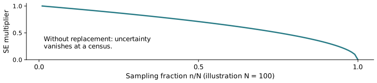
Finite-population correction and small-population example
The slide deck begins here; the notes place this topic after sample-size planning. PDF page numbers are preserved.
From point estimation to interval estimation
Central normal probabilities and critical values
Sampling distribution and confidence interval for one mean
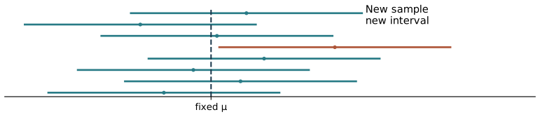
Derivation on notes p. 2; repeated-sampling interpretation on p. 3. A fixed observed interval does not assign a probability to the unknown parameter.
Estimated standard error and large-sample mean interval
Replacing sigma by S gives an approximate large-sample normal procedure, not an exactly normal statistic at n = 30. Notes p. 6 makes this distinction explicit.
Dietitian example
The problem and calculation use n = 100. The first line on slide PDF p. 37 says n = 50; this is a source typo. Notes p. 6 consistently uses n = 100 and obtains [0.70, 14.42] grams/day.
Interpreting confidence
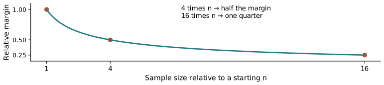
Confidence level, precision and interval width
Why sample variance uses n − 1
Notes p. 6 introduces estimated variability; p. 15 contains the full derivation.
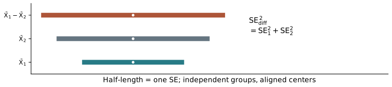
Difference between two independent population means
Estimated-SE normal inference is approximate; adequate sample sizes and independent groups are separate requirements.
Sampling distribution of a proportion
Blue-eyes probability example
For p = 0.09 and n = 613, the standard error is 0.011559 and the direct normal tail is about 0.0418. The values 0.0121 and 0.0564 on slide PDF pp. 61–62 are arithmetic errors. Notes p. 8 gives the corrected calculation and distinguishes it from a continuity-corrected count calculation.
Confidence interval for one proportion
Difference between two independent proportions
Bond-proposal example
Choosing a sample size and planning values
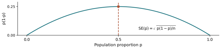
The notes explain the limits of the range/4 rule and why p = 1/2 gives conservative proportion planning.
95% confidence with a one-percentage-point margin
Additional Practice 1: one mean
This water-specimen question is additional course practice. Related slide sections: one-mean confidence intervals, interpretation and width.
Formula map, inverse calculations and final checks
These pages synthesize the chapter and add checks; they do not correspond to one slide range. The Chapter 6 sum tools on notes p. 14 connect to Chapter 6 slide PDF pp. 62–81.
Additional Problem 2: two means
This protein-concentration question is additional course practice. Use the two-means section, slide PDF pp. 46–53.
Additional Problem 3: one proportion
This usable-water-sample question is additional course practice. Related slides: sampling proportions pp. 54–62, proportion intervals pp. 63–64 and sample-size planning pp. 72–83.
Office-hours appendix
The existing office-hours appendix is preserved. It has no lecture-slide counterpart.